ファイル:Butterworth response.png

元のファイル (1,240 × 880 ピクセル、ファイルサイズ: 86キロバイト、MIME タイプ: image/png)
ウィキメディア・コモンズのファイルページにある説明を、以下に表示します。 |
概要
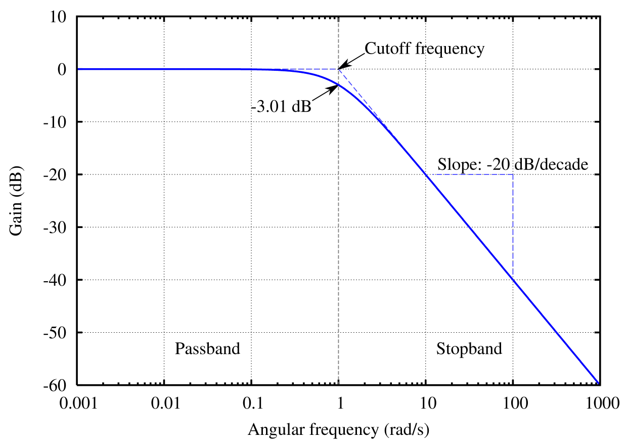
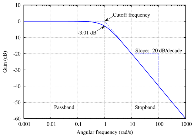
| 解説 | English: The frequency response of a Butterworth filter with logarithmic axes (Bode plot) and various labels. Cutoff frequency is normalized to 1 rad/s. Gain is normalized to 0 dB in the passband. Many orders on one plot: File:Butterworth orders.png. Version with no text available at File:Butterworth plain.png, though you should probably just modify the source code and regenerate it in your own language. See Wikipedia graph-making tips. Generated in gnuplot with the script below (save as butterworth.plt and then open in gnuplot). Then I opened the butterworth.ps file in a text editor to edit the line colors and linestyles, as per this description. This avoids needing to open in proprietary software, and really isn't that difficult (especially if you don't know the commands in the proprietary software either). ;-) Identify the lines easily by their color (the arrow is currently magenta and I want it to be black. Ah, there is the entry with 1 0 1, red + blue = magenta) or by using the gnuplot linestyle−1. (For instance, gnuplot's linestyle 3 corresponds to the ps file's /LT2.) Then you can edit the colors and dashes by hand. I changed the original: /LT0 { PL [] 1 0 0 DL } def /LT1 { PL [4 dl 2 dl] 0 1 0 DL } def /LT2 { PL [2 dl 3 dl] 0 0 1 DL } def /LT3 { PL [1 dl 1.5 dl] 1 0 1 DL } def into this: /LT0 { PL [] 0 0 1 DL } def /LT1 { PL [4 dl 2 dl] 0.5 0.5 0.5 DL } def /LT2 { PL [6 dl 3 dl] 0.3 0.3 1 DL } def /LT3 { PL [] 0 0 0 DL } def /LT4–/LT8 I left unchanged. (I don't know what they're used for anyway.) /LTw, /LTb, and /LTa are for the grid lines and such.To convert the PostScript file to PNG:
|
| 日付 | 2005年6月26日 (アップロード日) |
| 原典 | 投稿者自身による著作物 |
| 作者 | Omegatron |
| その他のバージョン |
|
| gnuplot source | click to expand set samples 2001 set terminal postscript enhanced landscape color lw 2 "Times-Roman" 20 set output "butterworth.ps" # Butterworth amplitude response and decibel calculation. n is the order, which is just 1 in this image. G(w,n) = 1 / (sqrt(1 + w**(2*n))) dB(x) = 20 * log10(abs(x)) # Gridlines set grid # Set x axis to logarithmic scale set logscale x 10 # Set range of x and y axes set xrange [0.001:1000] set yrange [-60:10] # Create x-axis tic marks once per decade (every multiple of 10) set xtics 10 # Use 10 x-axis minor divisions per major division set mxtics 10 # Axis labels set xlabel "Angular frequency (rad/s)" set ylabel "Gain (dB)" # No need for a key set nokey #0.1,-25 # Frequency response's line plotting style set style line 1 lt 1 lw 2 # Draw a separator between passband and stopband and label them set style line 2 lt 2 lw 1 set style arrow 2 nohead ls 2 set arrow 3 from 1,-60 to 1,10 as 2 # Label coordinates are relative to the graph window, not to the function, centered at the 1/4 and 3/4 width points set label 1 "Passband" at graph 0.25, graph 0.1 c set label 2 "Stopband" at graph 0.75, graph 0.1 c # Asymptote lines and slope lines are the same "arrow" style set style line 3 lt 3 lw 1 set style arrow 3 nohead ls 3 # Draw asymptote lines set arrow 1 from 1,0 to 1000,-60 as 3 set arrow 2 from .001,0 to 1,0 as 3 # -3 dB arrow style and arrow set style line 4 lt 4 lw 1 set style arrow 4 head filled size screen 0.02,15,45 ls 4 set arrow 4 from 2,3 to 1,0 as 4 # "Cutoff frequency" label uses same coordinates as the function set label 3 "Cutoff frequency" at 2,4 l # "-3 dB" label set arrow 5 from 0.5,-6 to 1,-3 as 4 set label 4 "-3.01 dB" at 0.5,-7 r # Draw slope lines and label set arrow 6 from 100,-20 to 12,-20 as 3 set arrow 7 from 100,-20 to 100,-39 as 3 set label 5 "Slope: -20 dB/decade" at 100,-18 c # Plot the filter response plot \ dB(G(x,1)) ls 1 title "1st-order response" |


 | このファイルのベクター画像 (SVG) が利用できます。 使う目的に対し、元画像よりもSVGがより優れている場合、SVG画像を使用して下さい。 File:Butterworth response.png → File:Butterworth response.svg |  |
ライセンス
- あなたは以下の条件に従う場合に限り、自由に
- 共有 – 本作品を複製、頒布、展示、実演できます。
- 再構成 – 二次的著作物を作成できます。
- あなたの従うべき条件は以下の通りです。
- 表示 – あなたは適切なクレジットを表示し、ライセンスへのリンクを提供し、変更があったらその旨を示さなければなりません。これらは合理的であればどのような方法で行っても構いませんが、許諾者があなたやあなたの利用行為を支持していると示唆するような方法は除きます。
- 継承 – もしあなたがこの作品をリミックスしたり、改変したり、加工した場合には、あなたはあなたの貢献部分を元の作品とこれと同一または互換性があるライセンスの下に頒布しなければなりません。
 | この文書は、フリーソフトウェア財団発行のGNUフリー文書利用許諾書 (GNU Free Documentation License) 1.2またはそれ以降のバージョンの規約に基づき、複製や再配布、改変が許可されます。不可変更部分、表紙、背表紙はありません。このライセンスの複製は、GNUフリー文書利用許諾書という章に含まれています。 |
ファイルの履歴
過去の版のファイルを表示するには、その版の日時をクリックしてください。
| 日付と時刻 | サムネイル | 寸法 | 利用者 | コメント | |
|---|---|---|---|---|---|
| 現在の版 | 2005年7月23日 (土) 17:45 | | 1,240 × 880 (86キロバイト) | Omegatron | split the cutoff frequency markers |
| 2005年7月23日 (土) 16:31 |  | 1,250 × 880 (92キロバイト) | Omegatron | Better butterworth filter response curve | |
| 2005年6月26日 (日) 19:54 |  | 250 × 220 (2キロバイト) | Omegatron | A graph or diagram made by User:Omegatron. (Uploaded with Wikimedia Commons.) Source: Created by User:Omegatron {{GFDL}}{{cc-by-sa-2.0}} Category:Diagrams\ |
ファイルの使用状況
以下のページがこのファイルを使用しています:
グローバルなファイル使用状況
以下に挙げる他のウィキがこの画像を使っています:
- be-tarask.wikipedia.org での使用状況
- de.wikipedia.org での使用状況
- eo.wikipedia.org での使用状況
- et.wikipedia.org での使用状況
- fr.wikipedia.org での使用状況
- hi.wikipedia.org での使用状況
- it.wikipedia.org での使用状況
- pl.wikipedia.org での使用状況
- pt.wikipedia.org での使用状況
- zh.wikipedia.org での使用状況